Mark Kong

The 15 puzzle is a well-known puzzle.  In this exercise, we constructed a simple solver for the puzzle through the Metropolis-Hastings algorithm.

A random walk will take a long time to solve a randomly chosen puzzle.  Indeed, for any board \(B\), the stationary distribution for this random walk is proportional to the function

\(f(B):=\begin{cases}2&\textrm{the blank space is in a corner}\\3&\textrm{the blank space is on an edge}\\4&\textrm{the blank space is in the middle}\end{cases}.\)

For any blank tile, there are \(15!\) ways to arrange the other tiles, half of which are solvable.  Then the proportion of the time we spend at the solved state is \(\frac{2}{2*4*\frac{15!}{2}+3*8*\frac{15!}{2}+4*4*\frac{15!}{2}}=\frac{1}{15 692 092 416 000}\).  I’m not sure how to use this to bound the expected amount of time it would take to solve the puzzle, but it does seem like it would take a long time.

We then applied the Metropolis-Hastings algorithm to generate moves in a 15-puzzle.  Letting \(d\) denote taxicab distance and \(B[i,j]\) denote the coordinates of the position that the piece at \((i,j)\) is supposed to be at, if we define the Hamiltonian

\(H(B):=\displaystyle \sum_{i,j=1}^{4}d(B[i,j], (i,j))*w(B[i,j])\)

where \(w\) is some weighting function, we can define a distribution on the set of all (solvable) boards we want to attain by

\(p(B)\propto e^{-H(B)}.\)

We used the weighting \(w(i,j)=\begin{cases}\frac{1}{8}&i,j=4\\1&\textrm{else.}\end{cases}\)

The choice of \(\frac{1}{8}\) was chosen as the sum of the width and height of the board; I have not tried to optimize this.

We run the algorithm on 100 randomly generated puzzles, and we can plot how long it takes to solve each puzzle.  We get the following graph:

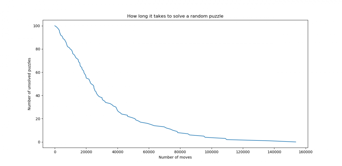
We observe that this decays faster than an exponential function.  From this, we conclude that positions reached after running this algorithm for many steps are more likely to be solved in fewer steps by this algorithm.  It is noted that typically, the number of steps the algorithm takes to solve the puzzle is of several orders of magnitude more than the shortest possible solution. It is not hard to do better by trying to optimize the weighting function or by adding a few parameters to the Hamiltonian and optimizing those parameters.  One can also do something more clever.

We did not go in either path. This is because the main point in this exercise is this:  our extremely simple and nearly “effortless” Hamiltonian gave a solution in a reasonable time, in stark contrast to the random walk that was impractical, or a more sophisticated approach that requires much more thought.