Phil Speegle
In this exercise, we applied the Metropolis-Hastings algorithm to find the extrema of functions with three variables. Although this seems trivial, some functions such as the well-known Rosenbrock Function has a global minimum which is notoriously difficult for an optimization algorithm to converge to. This function, defined as $R(x,y) = (1-x^2)+100(y-x^2)^2$ has a parabolic valley with values quite close to the global minimum at $(1,1)$. As such, algorithms that try and “seek” the global minimum often confuse this valley for the global minimum and get stuck.
Instead of working with the Rosenbrock function directly, we worked with function
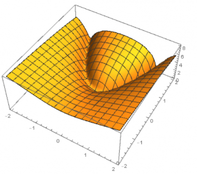
\[f(x,y) = \log (1+R(x,y)).\]
The idea behind the implementation of the Metropolis-Hastings algorithm is to introduce an element of randomness to avoid getting stuck in local extrema.
We’ll start at a point $(x,y)$, specified by the user, and feed the algorithm a random point close by, $(x’,y’)$. The algorithm can either decide to move to the new point with probability $p$, or stay at the old point with probability $1-p$. This probability is determined by a function which increases $p$ if $f(x’,y’) < f(x,y)$. In this way, it is more likely that the algorithm “accepts” new values that decrease the function than values that increase it. However, sometimes the algorithm will accept a new value that increases the function, which is useful for getting out of pesky local minimums.
Here is exactly how it’s done. The code was written in Wolfram Mathematica and is not too hard, so follow along on your own device if you want to see the magic happen yourself!
First, we must define our function $f$ we’re going to find the minimum of. Here,
f[{x_, y_}] := Log[(1 - x)^2 + 100 (y - x^2)^2 + 1]
We then fix a negative parameter $s$, and a starting point $(x,y)$.
s = -1;
Then we start a walk on ${\mathbb R}^2$. This is done by sampling a vector $Z=(r_1,r_2)$, where $r_1,r_2$ are independent standard normal RVs. We move from $(x,y)$ to $(x,y)+Z$ with probability
\[ \min (\frac{e^{s f((x,y)+Z)}}{e^{s f(x,y)}},1).\]
Otherwise, it stays put. Since $s<0$, whenever $f((x,y)+Z)<f(x,y)$, we move, and otherwise we move with probability less than one. This last part is what allows to eventually leave local minima. Here’s the code:
update [{x_, y_}] :=
Module[{r1 = Random[NormalDistribution[0, 1]],
r2 = Random[NormalDistribution[0, 1]]},
RandomChoice[{Min[E^(s*f[{x + r1, y + r2}])/E^(s*f[{x, y}]), 1],
1 - Min[E^(s*f[{x + r1, y + r2}])/E^(s*f[{x, y}]), 1]} -> {{x +
r1, y + r2}, {x, y}}]]
The parameter s can be made whatever you want. In some implementations, this parameter is adaptively changed (made more negative) in order to limit the movement after a large number of steps (think why!). Play around with it to see what happens. Similarly, you can change the variance of r1 and r2, but you generally shouldn’t make it too high.
Print["The min of f(x,y) is ",
Min[Map[f, NestList[update, {-10., -10.}, 10000]]]]
Finally, we’ll call the update function 10,000 times and see if it converges correctly. If you want, you can increase the amount of times you call the function and the starting point.
The min of f(x,y) is 0.0000286096
Unless you’re incredibly unlucky, you’ll get something like this.
Seeing as the minimum of the function is indeed zero, I’d say the algorithm did a great job of calculating it. The cool thing is, even if you start on a point that’s on the valley, the algorithm will eventually escape the local minimums if you call the update function enough times!
To illustrate the algorithm working, we are now going to create a fun animation that showcases its path. Here is the code for it:
list = NestList[update, {-12., -12.}, 600]; newlist =
Table[Take[list, j], {j, 1, Length[list]}];
ListAnimate[
Map[Show[{DensityPlot[f[{t1, t2}], {t1, -17, 17}, {t2, -17, 17}],
ListPlot[#, PlotStyle -> {PointSize[Small], Green},
Joined -> True]}] &, newlist]]
Note that the animation references the update function shown above. Let’s see it in action!
What we see is a heatmap of $f$, and the path of our walk ending near the global minimum. If you ran it yourself, you most likely got a different path, but from my experience, 1000 steps usually get you pretty close to target. You can run it multiple times from various initial points to empirically verify you have found the global minimum.
On a final note, it is always fun to experiment with functions other than the Rosenbrock function; the algorithm will still work. Try inputting a function with many global minimums, or maybe try and modify it to find a global maximum instead (it’s not too hard!)
The motivation for this project comes from here
